Anne Reinarz Durham University
Fast Multipole
Fast Multipole
L. Greengard, V. Rokhlin: A fast algorithm for particle simulations. J. Comp. Phys., 73, 1987.
C. R. Anderson: An implementation of the Fast Multipole Method without multipoles.. SIAM J. Sci. Stat. Comput. 13(4), 1992.
Complexity of Fast Multipole
Lets do a computation with $N = 10^6$ particles assuming that $N$ computations take 1 hour
- $O(N)$ algorithm $\to$ 1 hour
- $O(N\log N)$ algorithm $\to$ $14$ hours
- $O(N^2)$ algorithm $\to$ $10^{6}$ hours, or 114 years
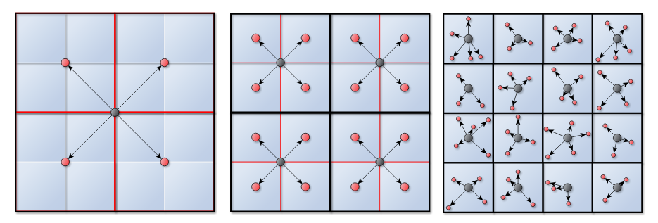
Fast Multipole Method:
- define a pseudo particle (as in Barnes-Hut) for each cell $\to$ accumulated mass located in centre of mass
- force computation:
- between particles in the same or in adjacent cells: add particle–particle force
- between particles in separated cells:
- add forces between corresponding pseudo-particles;
- accumulate that force to all particles of a pseudo particle
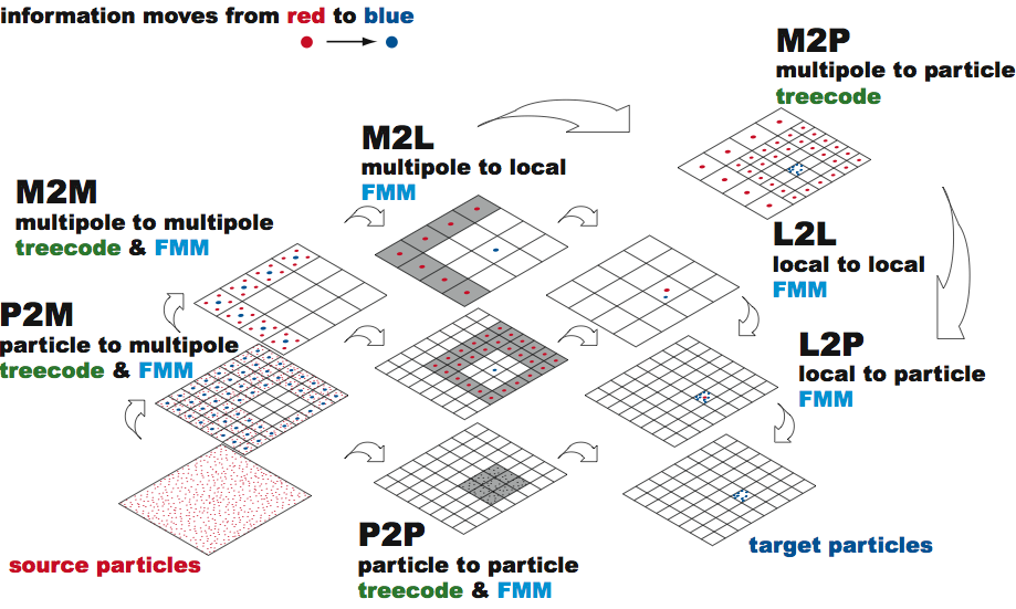
Fast Multipole Method
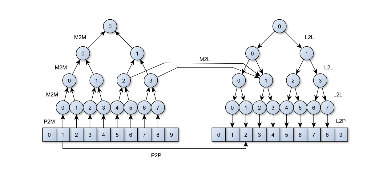
Image from the Master thesis of Fabio Gratl
Required kernels
P2M: Particle to Multipole
-
in Barnes-Hut this involved summing the mass, and computing the center of mass
$\to$ locate centre of mass $X_l := \frac{1}{M_l} \sum_j m^{(l)}_j x^{(l)}_j$
$\to$ accumulated mass $M_l := \sum_j m^{(l)}_j $
-
in FMM: use multipole expansion
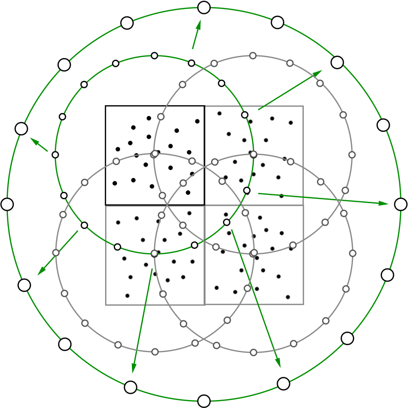
Constructing Multipoles (M2M/P2M)
2 Approaches:
Original Approach of Greengard/Rohlkin, 1987
- similar concept as Taylor series
- complicated to derive, esp. in 3D (spherical harmonics)
- complicated formula for hierarchical assembly
Constructing Multipoles (M2M/P2M)
2 Approaches:
Or: inner/outer ring approximations by Anderson, 1992
- derived via numerical integration of an integral formula
- uniform interaction with child and remote boxes
- hierarchical assembly via evaluation of potentials at integration points
Anderson’s method
Fundamental idea: represent potential via a surface integral
\[\Psi_a (\vec{x}) = \int\limits_{S^2} g( a \vec{s} ) \left( \sum\limits_{n=0}^\infty \left( \frac{a}{r} \right)^{n+1} Q_n(\vec{s} \cdot \vec{x}_p ) \right) ds\]- in spherical coordinates $\vec{x} = ( r, \theta, \psi)$,
- with suitable $Q_n$ (charges or mass)
- $\vec{x}_p = ( 1, \theta, \psi)$,
- $g( a \vec{s} )$ the potential on a sphere of radius $a$ that contains all particles
Anderson’s method
- and use numerical integration to compute the integral
- using $K$ integration points $\vec{s}_i$ on the sphere $S^2$ (weights $w_i$)
- and choosing $M$ relative to accuracy of integration rule
Anderson’s method
\[\Psi_a (\vec{x}) \approx \sum w_i \, g( a \vec{s}_i ) \left( \sum\limits_n \left( \frac{a}{r} \right)^{n+1} Q_n(\vec{s}_i \cdot \vec{x}_p ) \right)\]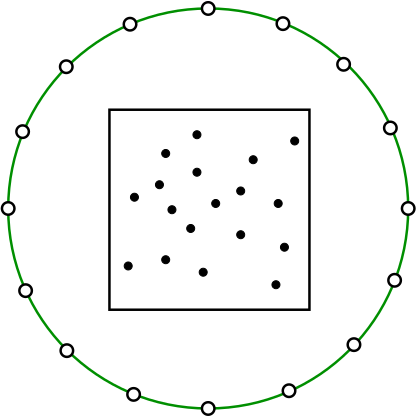 </img>
Required kernels
P2M: Particle to multipole
- Original approach: compute multipole expansion, i.e. “Taylor-series”
- With Anderson’s method: compute surface integral with numerical integration
- approximate potential caused by all particles of the current box
- evaluate and accumulate particle potentials at positions $a \vec{s}_i $ to obtain values $g( a \vec{s}_i )$
Required kernels
M2M: Multipole to Multipole
 </img>
Upward Pass
Required kernels
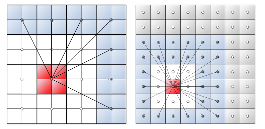
M2L: Multipole to Local
-
box–box interactions occur at multiple levels
$\to$ as particles are part of all parent/grand-parent pseudo particles, the interaction between two particles might be captured by box–box interactions on multiple levels
$\Rightarrow$ make sure that each particle–particle interaction is considered exactly once!
Required kernels
M2L: Multipole to Local
- force computation between pseudo particles occurs, if:
- pseudo particles are not in cells that are direct neighbours (requires particle–particle interaction, no approximation via pseudo particles allowed)
- interaction between the boxes that contain those pseudo particles is not considered on coarser levels
$\to$ considers comparably few interactions on each level that are ``nearby’’ but neither direct neighbours nor too far away
“Horizontal” Pass
 </img>
“Horizontal” Pass
Compute forces – far-field (M2L)
- For a cell $C_l$:
- compute interactions with cells that are not direct neighbors and have not been considered on previous levels
Compute forces – near-field (P2P)
- For a cell $C_L$ on the finest level $L$:
- compute particle to particle forces for neighboring cells and within the cell
Required kernels: Downward Pass
- For a leaf cell:
- compute local to particle interaction (L2P)
- For any other cells:
- compute a local to local interaction (L2L)
Required kernels: Downward Pass
 </img>
Fast Multipole Method – Summary
R. Yokota:
 </img>
Fast Multipole Method – Summary
-
Initialization: Choose a number of levels such that there are approx. $s$ particles per cell at the finest level. $\to$ $N/s$ cells
-
Upward Pass: Beginning at the finest level create multipole expansions (P2M). Expansions cells at higher levels formed by the merging (M2M).
-
Downward Pass: Compute the far-field (M2L) and near-field (P2P). Convert the multipole expansion into a local expansion about the centers of all cells (L2L/L2P).
Fast Multipole Method – Summary
Accuracy:
-
depends on accuracy of integration rule
$\to$ determined by number of integration points
-
in practice: can be increased to allow approximations that are accurate up to machine precision
Fast Multipole Method – Summary
Complexity:
-
computation of box-approximations, i.e., all $g( a \vec{s}_i )$
$\to$ constant effort per box (leaf and inner boxes)
$\to$ thus $O(N_\text{B})$ effort ($N_\text{B}$ boxes);
- if max. number of particles per box is constant then $O(N)$ for $N$ particles
-
computation of forces
$\to$ multilevel algorithms leads to $O(N)$ effort
Comparison of Barnes-Hut and FMM
Approximate potential of sets/clusters of particles
- Barnes-Hut
- pseudo particles in tree cells
- $\theta$-criterion to determine far-field
- Fast Multipole
- higher-order representations necessary!
- no $\theta$-criterion to tune accuracy (instead choose number of terms in expansion)
Comparison of Barnes-Hut and FMM
Hierarchical computation of box potentials
- Barnes-Hut
- combine pseudo particles in child cells
- Fast Multipole
- generate high order box potentials
- (accumulate approximate potentials of child boxes to approximate potential of parent box $\to$ needs to be derived for high-order representation)